The idea for this post began on a random day, during a walk with a friend through Barcelona’s Eixample district (Eixample in Catalan, Ensanche in Spanish). This iconic grid layout features chamfered corners, which raises an interesting geometric question:

• We walk a longer distance if traveling along a straight line.
• We walk a shorter distance if moving diagonally—provided we choose our path wisely.

Since my academic background in mathematics included a statistics course I now only vaguely recall, I decided to challenge myself: does this chamfered design actually reduce the average distance traveled across the grid?

(Also, I’ve just finished my undergraduate studies, it's summer, and I’m desperate to waste my free time on pointless side projects.)

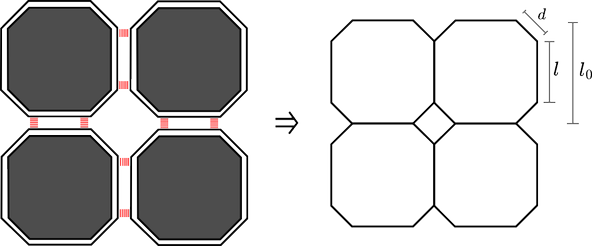
The grid model will be characterized by three parameters:

• $l_0$: the side length of the original square blocks,
• $l$: the side length after the chamfer is applied,
• $d$: the chamfer length.

---

The Most Efficient Path in the Grid

Let’s simplify the problem. At intersections, we can conceptually merge the streets, since the exact layout of crossroads and lanes doesn't affect our analysis. Thus, the grid can be abstracted as follows:

On a regular grid, to go from point $(a_1, b_1)$ to $(a_2, b_2)$, many shortest paths exist, all zigzagging within the rectangle defined by those two points. However, with chamfers, this set of efficient paths narrows. The chamfers allow for a more diagonal-like movement, a sort of diagonalization.

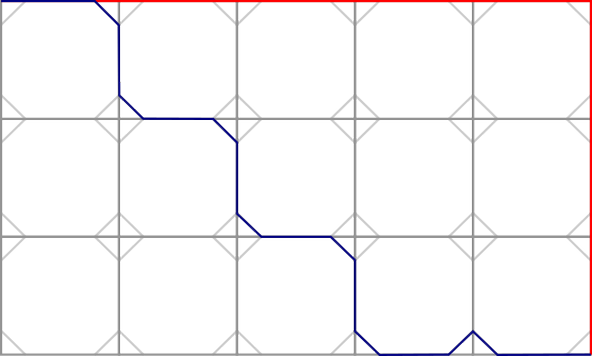
In the figure above, the red path shows the standard Manhattan distance, while the blue path leverages the chamfered corners.

Given a displacement of $(a, b)$, where $b \ge a$, the corresponding distances are:

$$ d_m = (a + b) l_0 \quad \text{and} \quad d_c = (a + b) l + 2(b - 1)d + (l_0 - l) \approx (a + b) l + 2 b d $$

From here, we’ll explore two ways to analyze the efficiency of chamfers: analytically and numerically.

---

Analytical Approach

Assume the grid is sufficiently large, so we can use a continuous model for simplicity. We analyze the ratio:

$$ f(a, b) = \frac{d_c}{d_m} = \frac{(a + b)l + 2bd}{(a + b)l_0} $$

If $f(a, b) < 1$, then the chamfered grid is more efficient. Interestingly, this function primarily depends on the ratio $r = \frac{a}{b}$, since:

$$ f(r) = \frac{l}{l_0} + \frac{2d}{(1 + r)l_0} $$

Knowing $d = \frac{\sqrt{2}}{2}(l_0 - l)$, we substitute and get:

$$ f(r) = \frac{l}{l_0} + \frac{\sqrt{2}}{1 + r} \left(1 - \frac{l}{l_0}\right) $$

To find the cases when $f(r) < 1$, we solve:

$$ \frac{\sqrt{2}}{1 + r} \left(1 - \frac{l}{l_0} \right) < 1 - \frac{l}{l_0} \Rightarrow r > \sqrt{2} - 1 $$

Remarkably, the threshold ratio is independent of the specific chamfer length $d$.

Distribution of Path Ratios

To quantify how often $r > \sqrt{2} - 1$, consider two points randomly placed in the unit square:

$$ \mathbf{x}_i, \mathbf{y}_i \sim U(0, 1) $$

The displacement $(a, b) = (|x_1 - x_2|, |y_1 - y_2|)$, assuming $a \le b$, has the probability density:

$$ p(a, b) = 8(1 - a)(1 - b) $$

Thus, for computing the probability distribution of the ratio $r = \frac{a}{b}$ we perform the following change of variables: $$ r = \frac{a}{b}, \quad b = b, \quad J = \frac{\partial(a,b)}{\partial(r,b)} = \begin{vmatrix} b & 0 \ r & 1 \end{vmatrix} = b $$

And the resulting probability density function becomes:

$$ p(r) = \int_0^1 8 (1 - r b)(1 - b) bdb = \frac{4}{3} - \frac{2}{3} r $$

Now compute the probability that $r > \sqrt{2} - 1$:

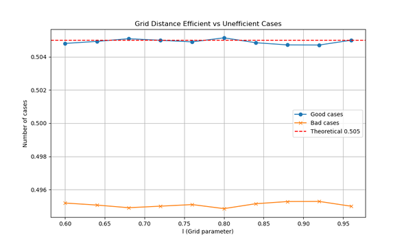
$$ P(r > \sqrt{2} - 1) = \int_{\sqrt{2} - 1}^{1} \left(\frac{4}{3} - \frac{2}{3}r\right) dr = \frac{10}{3} - 2\sqrt{2} \approx 0.505 $$

So, slightly more than half the time, a chamfered grid is more efficient.

Expected Value Comparison

Let’s compute the expected distances under this uniform distribution:

For the regular grid:

$$ \langle d_m \rangle = \int_{0}^{1} \int_{0}^{b} 8(1 - a)(1 - b)(a + b)l_0 da db = \frac{2}{3} l_0 $$

For the chamfered grid:

$$ \langle d_c \rangle = \int_{0}^{1} \int_{0}^{b} 8(1 - a)(1 - b)[(a + b)l + 2bd] da db = \frac{2}{3}l + \frac{14}{15}d = \frac{2}{3}l + \frac{7\sqrt{2}}{15}(l_0 - l) $$

Taking the ratio:

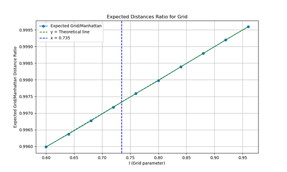
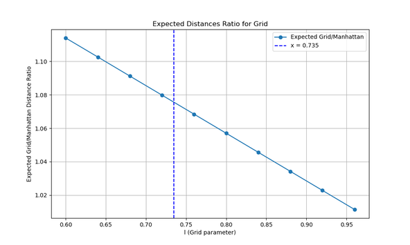
$$ \frac{\langle d_c \rangle}{\langle d_m \rangle} = \frac{7\sqrt{2}}{10} + \left(1 - \frac{7\sqrt{2}}{10} \right)\frac{l}{l_0} \approx 0.98995 + (1 - 0.98995)\frac{l}{l_0} $$

As expected, this ratio decreases as the chamfer becomes more pronounced (i.e., as $l/l_0$ decreases).

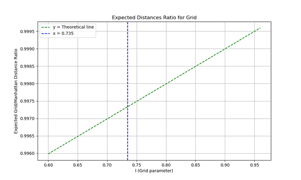
The vertical line represents the actual value of $\frac{l}{l_0} = 0.735$ in Barcelona's Eixample.

---

Numerical Approach

To simulate this behavior, we define a large grid and randomly choose pairs of points. Numerical simulations allow more flexibility, avoiding the complexity of analytical probability densities.

First, define grid size and sample count:

N = 1000000  # Grid size
M = 1000000  # Number of samples

Define distance functions:

def to_abcoord(p1, p2):
    return abs(p1[0] - p2[0]), abs(p1[1] - p2[1])

def dist_manhattan(a, b):
    return a + b

def dist_eixample(a, b, l):
    d = np.sqrt(2)/2 * (1 - l)
    if a == 0 and b == 0:
        return 0
    if a == b:
        return l*(a + b) + d*(2*a - 1) + (1 - l)
    if a < b:
        return l*(a + b) + 2*d*a + 2*d*(b - a - 1) + (1 - l)
    return dist_eixample(b, a, l)

Now run simulations:

def eixample():
    stats = []
    for j in range(10):
        l = 0.6 + j * 0.04
        samples = []
        for _ in range(M):
            p1 = np.random.randint(0, N, size=2)
            p2 = np.random.randint(0, N, size=2)
            a, b = to_abcoord(p1, p2)
            d_m = dist_manhattan(a, b)
            d_e = dist_eixample(a, b, l)
            samples.append((d_m, d_e, d_e < d_m))
        good_cases = sum(s[2] for s in samples)
        expected_m = sum(s[0] for s in samples) / M
        expected_e = sum(s[1] for s in samples) / M
        stats.append((l, good_cases/M, 1 - good_cases/M, expected_e/expected_m))

    # Plotting results
    ...

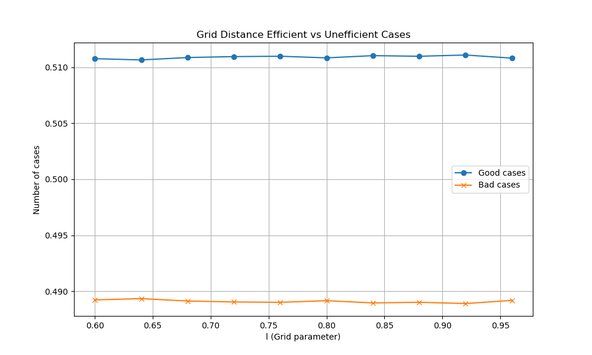
The plots generated confirm our expectations:

• The first plot shows how often chamfers provide a shorter route.
• The second plot shows that the expected distance improves linearly with increasing chamfer.

---

Bonus: Other global shapes

So far, our analysis has assumed the overall shape of the grid is square. But what happens if we change that? Let’s explore two interesting alternatives: the circle and the rectangle.

The Circle

In this scenario, we actually improve our results. When the global shape is circular, chamfered corners become even more efficient. This makes intuitive sense, since random paths within a circle are more likely to form diagonals rather than long vertical or horizontal stretches.

Here’s how the graphs change:

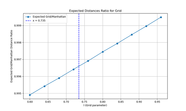
As you can see, both the frequency of improved paths and the average distance ratio benefit from the circular boundary.

The Rectangle

Now let’s consider a very different case: a rectangular grid. Take, for instance, the iconic Manhattan island, modeled as a grid roughly 15 avenues wide and 150 streets long.

What if we applied chamfered corners to Manhattan?

Intuitively, we might expect chamfers to be counterproductive here. Long, straight paths dominate in such elongated grids, and chamfers tend to favor diagonal movement. In this context, diagonalization offers little benefit.

And the data confirms our intuition: only about 14% of paths improve with chamfers.

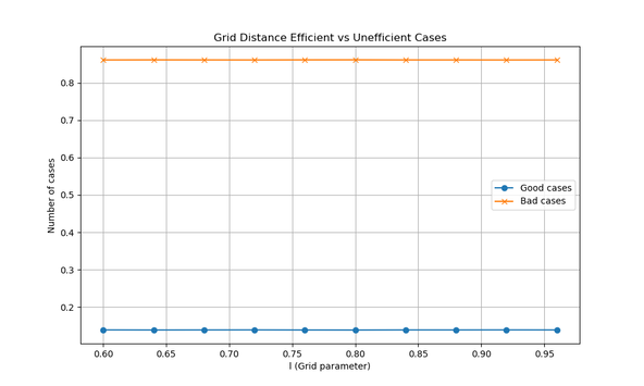
In conclusion, chamfers shine in square and circular layouts, but it loses its point on elongated rectangular grids.

---

I’m planning a follow-up post about the Eixample, this time exploring some of its historical and architectural curiosities. After living and studying in Barcelona for four years, I’ve had countless walks through this beautiful urban masterpiece, and there’s a lot more to share beyond the math.